Code
library(tidyverse)
library(tidytext)
library(malaytextr)
library(lubridate)
library(ggrepel)
library(showtext)
library(ggtext)

## Load font
font_add_google("Roboto", "Roboto")
showtext_auto()Using malaytextr & tidytext
Zahier Nasrudin
January 19, 2023
The dataset has been uploaded to my Github repository and is available for download, so you can use it to load the file for this analysis:
politic <- read_csv("https://github.com/zahiernasrudin/datasets/raw/main/politics.csv")


## set theme

theme_set(theme_minimal(base_family = "Roboto") +
            theme(plot.title = element_text(size = 40, family = "Roboto", face = "bold"),
                  legend.title=element_blank(), legend.text = element_text(size = 25),
                  plot.subtitle = element_markdown(size = 27, family = "Roboto"),
                  plot.caption = element_markdown(size = 15, family = "Roboto"),
                  axis.text = element_text(size = 20, family = "Roboto"),
                  axis.title = element_text(size = 25),
plot.caption.position = "plot"))We will remove the “RT” prefix from the tweets as part of the pre-processing stage. This prefix is frequently used at the start of the tweet text to indicate that the tweet is a retweet. Removing the “RT” prefix will ensure that tweet text we evaluate is original and not a re-post of the same tweet.
The tweets will first be categorized based on these hashtags
The date column will be reformatted.
## Categorize data
pn <- politic2 %>%
  filter(str_detect(text, "#perikatan|#Perikatan|#PERIKATAN")) %>%
  mutate(Party = "#perikatannasional")

bn <- politic2 %>%
  filter(str_detect(text, "#barisann|#Barisan|#BARISAN")) %>%
  mutate(Party = "#barisannasional")

ph <- politic2 %>%
  filter(str_detect(text, "#pakatan|#Pakatan|#PAKATAN")) %>%
  mutate(Party = "#pakatanharapan")

## Recombine dataset
politic2 <- bind_rows(pn, bn, ph)

## Change to date
politic2 <- politic2 %>%
  mutate(DATE = as_date(created_at))

## To factor
politic2 <- politic2 %>%
  mutate(Party = factor(Party, level = c('#pakatanharapan',
                                         '#perikatannasional',
'#barisannasional')))A graph displaying the total number of tweets using the hashtags #pakatanharapan, #barisannasional, and #perikatannasional. This graph gives a general overview of the volume of the tweets connected to these hashtags in the lead-up to Malaysia’s 15th General Election
politic2 %>%
  ## Count tweets by party
  count(DATE, Party) %>%
  ggplot(aes(x = DATE, y = n, colour = Party)) +
  geom_line() +
  ## Add notations
  geom_text_repel(data = politic2 %>%
                    filter(DATE == as_date("2022-11-05"),
                           Party == "#pakatanharapan") %>%
                    slice(1),
                  aes(x = as_date("2022-11-05"),
                      y = 350, label = "Nominations"),
                  max.overlaps = 1,
                  nudge_x = 4, nudge_y = 0.003, show.legend = F,
                  size = 8,
                  family = "Roboto") +
  labs(x = "",
       y = "Total Tweets",
       title = "Number of tweets",
       subtitle =  paste("From", min(politic2$DATE), "to",max(politic2$DATE)),
       caption = "by zahiernasrudin") +
scale_colour_manual(values = c("#17BEBB", "#2e282a", "#EDB88B")) 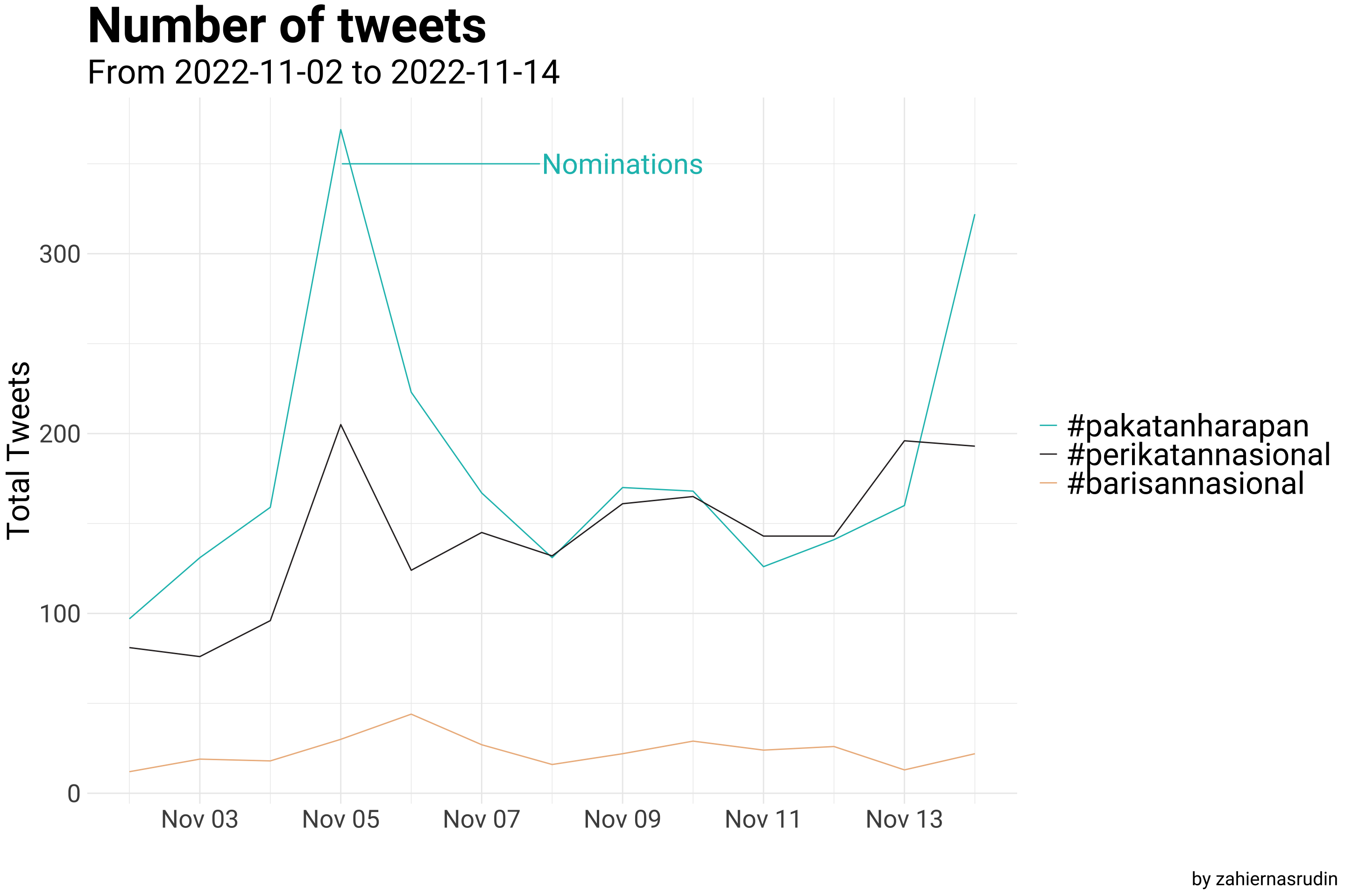
Additionally, the graph below is visualizing the distribution of tweets among Twitter users for the hashtags #pakatanharapan, #barisannasional, and #perikatannasional. This graph will demonstrate how Twitter users are participating in the political conversation in the lead up to Malaysia’s 15th General Election. It is important to keep in mind that the #barisannasional hashtag may have less Twitter users mentioning them comparatively, giving insights into its influence and scope.
politic2 %>%
  group_by(Party) %>%
  summarize(Total_user = n_distinct(id))  %>%
  mutate(Party = fct_reorder(Party, Total_user)) %>%
  ggplot(aes(x = Party, y = Total_user, fill = Party)) +
  geom_col(width = 0.3, show.legend = F) +
  geom_text(mapping=aes(label= Total_user, x = Party),
            size=7, family = "Roboto", hjust = -0.5) +
  scale_y_continuous(expand = c(0,0), limits=c(0,2600)) +
  coord_flip() +
  labs(x = "",
       y = "Total Users",
       title = "Number of unique Twitter users",
       caption = "by zahiernasrudin") +

scale_fill_manual(values = c("#EDB88B","#2e282a", "#17BEBB")) 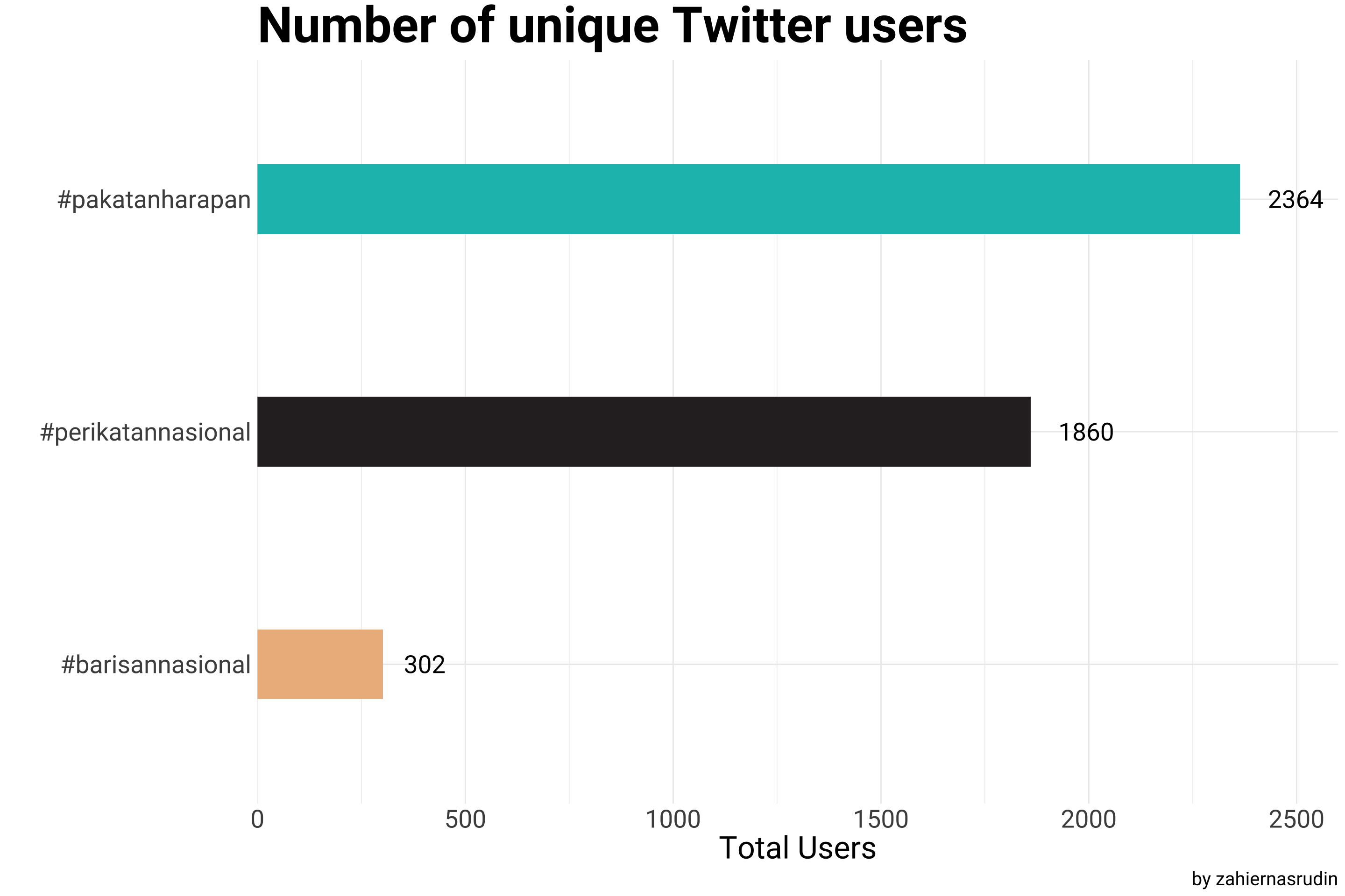
The tweets will then be split into individual tokens. Then, we will extract the positive and negative words. We can accomplish this by using the malaytextr package, which has a list of sentiments that can be used for this purpose.
A graph below is displaying the distribution of positive and negative words, separated by the hashtags, providing a visual representation of the overall sentiment of tweets mentioning #pakatanharapan, #barisannasional, and #perikatannasional. And how the word “rasuah” is being used within the hashtags; this is providing insights on the extent of corruption being discussed among these hashtags and among the users of these hashtags.
## Token & count sentiment words

count_sentiment <- politic2 %>%
  unnest_tokens(word, text) %>%
  inner_join(sentiment_general, by = c("word" =  "Word")) %>%
  count(word, Sentiment, Party,sort = TRUE) %>%
  ungroup()

## For Pakatan Harapn

count_sentiment %>%
  filter(Party == "#pakatanharapan") %>%
  group_by(Party, Sentiment) %>%
  slice_max(n, n = 10) %>%
  mutate(word = reorder(word, n)) %>%
  ggplot(aes(x = word, y = n, fill = Party)) +
  geom_col(width = 0.8, show.legend = F) +
  facet_wrap(~Sentiment, scales = "free_y") +coord_flip() +
  scale_fill_manual(values = c("#17BEBB")) +
   labs(x = "",
       y = "Total",
       title = "Words related to #pakatanharapan",
caption = "by zahiernasrudin") 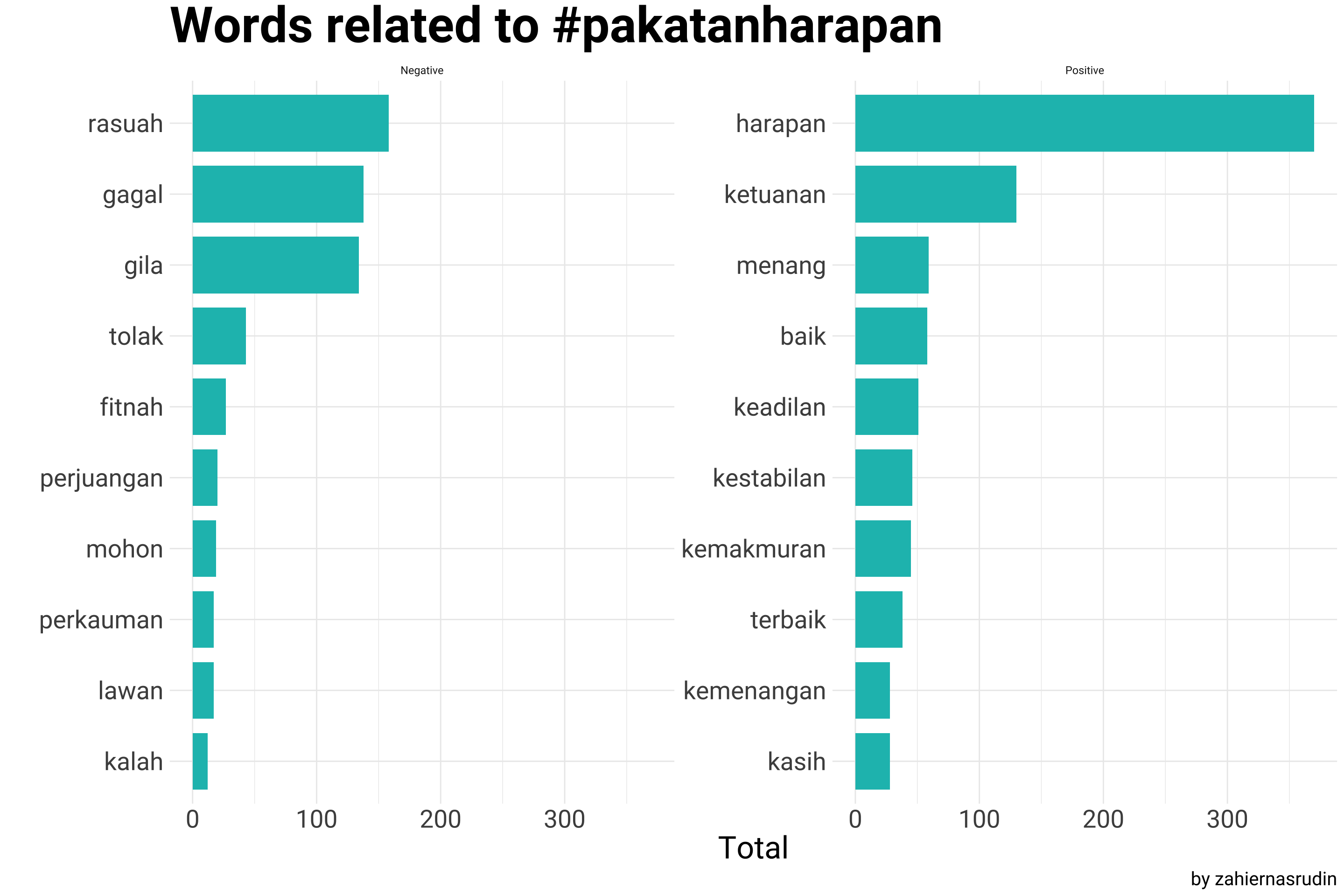
## For Perikatan Nasional

count_sentiment %>%
  filter(Party == "#perikatannasional") %>%
    group_by(Party, Sentiment) %>%
  slice_max(n, n = 10) %>%
  mutate(word = reorder(word, n)) %>%
  ggplot(aes(x = word, y = n, fill = Party)) +
  geom_col(width = 0.8, show.legend = F) +
  facet_wrap(~Sentiment, scales = "free") +
  coord_flip() +
  scale_fill_manual(values = c("#2e282a")) +
   labs(x = "",
       y = "Total",
       title = "Words related to #perikatannasional",
caption = "by zahiernasrudin") 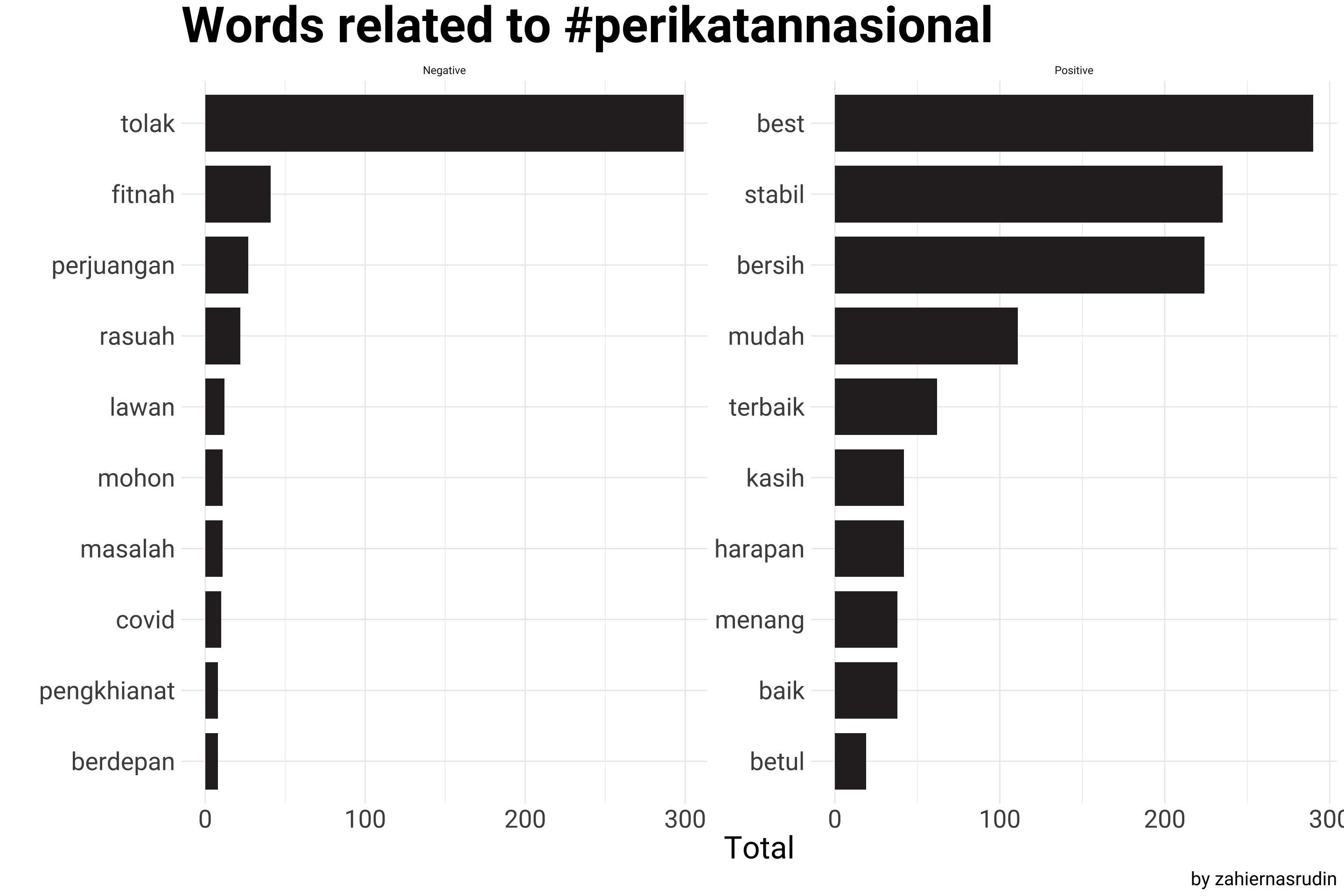
ggsave("img/sentiment_pn.jpeg",
       width = 8, height = 4)


## For Barisan nasional

count_sentiment %>%
  filter(Party == "#barisannasional") %>%
  group_by(Party, Sentiment) %>%
  slice_max(n, n = 10) %>%
  mutate(word = reorder(word, n)) %>%
  ggplot(aes(x = word, y = n, fill = Party)) +
  geom_col(width = 0.8, show.legend = F) +
  facet_wrap(~Sentiment, scales = "free") +
  coord_flip() +
  scale_fill_manual(values = c("#EDB88B")) +
   labs(x = "",
       y = "Total",
       title = "Words related to #barisannasional",
caption = "by zahiernasrudin") 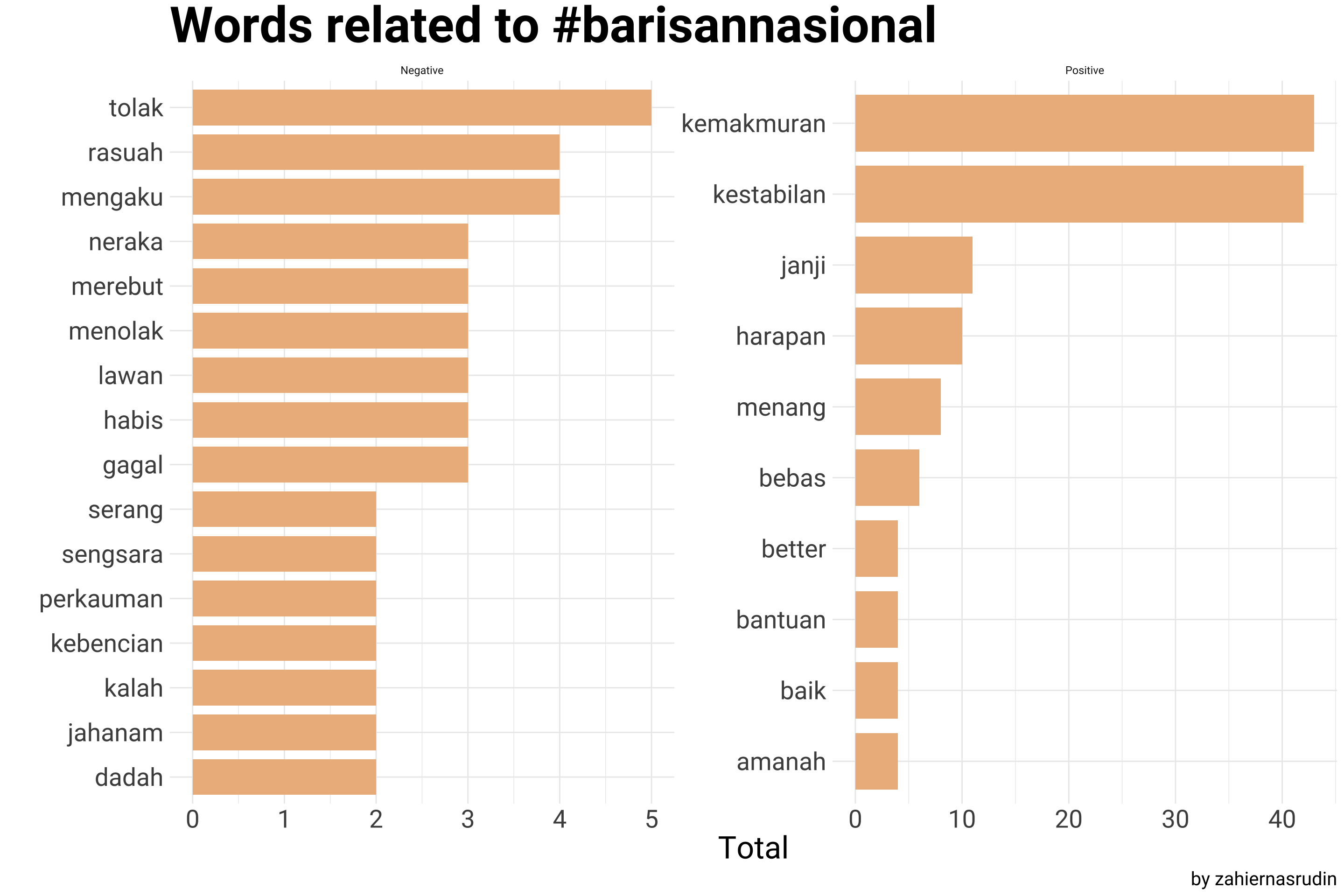
After performing a word-count analysis on the tweets, we will then take our analysis further by using bigrams. By doing this, we will be able to detect common phrases and expressions used in the tweets. In this analysis, we will be focusing on the term “rasuah”, by identifying bigrams that contain this word and to analyse their usage among the tweets that mention the hashtags #pakatanharapan, #barisannasional, and #perikatannasional in the lead-up to the 15th General Election of Malaysia. This will provide insights on how the word “rasuah” is being used in context within the political conversation on Twitter.
## Calculate bigram
ngram_ph <- ph %>%
## remove url & symbols from tweets
mutate(text = remove_url(text),
text = str_remove_all(text, "&|(#[^ ]*)")) %>%
unnest_tokens(word, text, token = "ngrams", n = 2) %>%
count(Party, word, sort = TRUE) %>%
filter(!is.na(word))
## Separate two words
ngram_ph_sep <- ngram_ph %>%
separate(word, c("word1", "word2"), sep = " ")
## Remove stop words
ngram_ph_sep <- ngram_ph_sep %>%
filter(!word1 %in% malaystopwords$stopwords) %>%
filter(!word2 %in% malaystopwords$stopwords)
# new bigram counts:
ngram_ph <- ngram_ph_sep %>%
unite(word, word1, word2, sep = " ")
ngram_ph %>%
filter(str_detect(word, "rasuah")) %>%
group_by(Party) %>%
slice_max(n, n = 4) %>%
ungroup() %>%
ggplot(aes(x = fct_reorder(word, n), y = n)) +
geom_col(width = 0.8, show.legend = F, fill = "#17BEBB") +
scale_y_continuous(expand = c(0,1), limits=c(0,150)) +
coord_flip() +
labs(x = "",
y = "Total",
title = "Word rasuah related to #pakatanharapan",
caption = "by zahiernasrudin")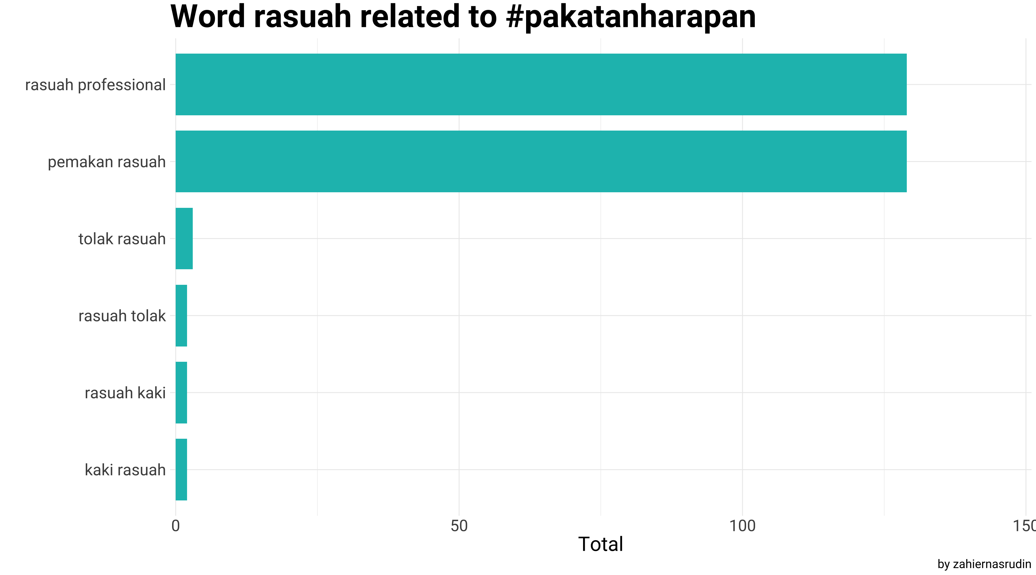
## Same step as in PH
ngram_pn <- pn %>%
mutate(text = remove_url(text),
text = str_remove_all(text, "&|(#[^ ]*)")) %>%
unnest_tokens(word, text, token = "ngrams", n = 2) %>%
count(Party, word, sort = TRUE) %>%
filter(!is.na(word))
ngram_pn_sep <- ngram_pn %>%
separate(word, c("word1", "word2"), sep = " ")
ngram_pn_sep <- ngram_pn_sep %>%
filter(!word1 %in% malaystopwords$stopwords) %>%
filter(!word2 %in% malaystopwords$stopwords)
# new bigram counts:
ngram_pn <- ngram_pn_sep %>%
unite(word, word1, word2, sep = " ")
ngram_pn %>%
filter(str_detect(word, "rasuah")) %>%
group_by(Party) %>%
slice_max(n, n = 4, with_ties = F) %>%
ungroup() %>%
ggplot(aes(x = fct_reorder(word, n), y = n)) +
geom_col(width = 0.8, show.legend = F, fill = "#2e282a") +
scale_y_continuous(expand = c(0,0), limits=c(0,7)) +
coord_flip() +
labs(x = "",
y = "Total",
title = "Word rasuah related to #perikatannasional",
caption = "by zahiernasrudin")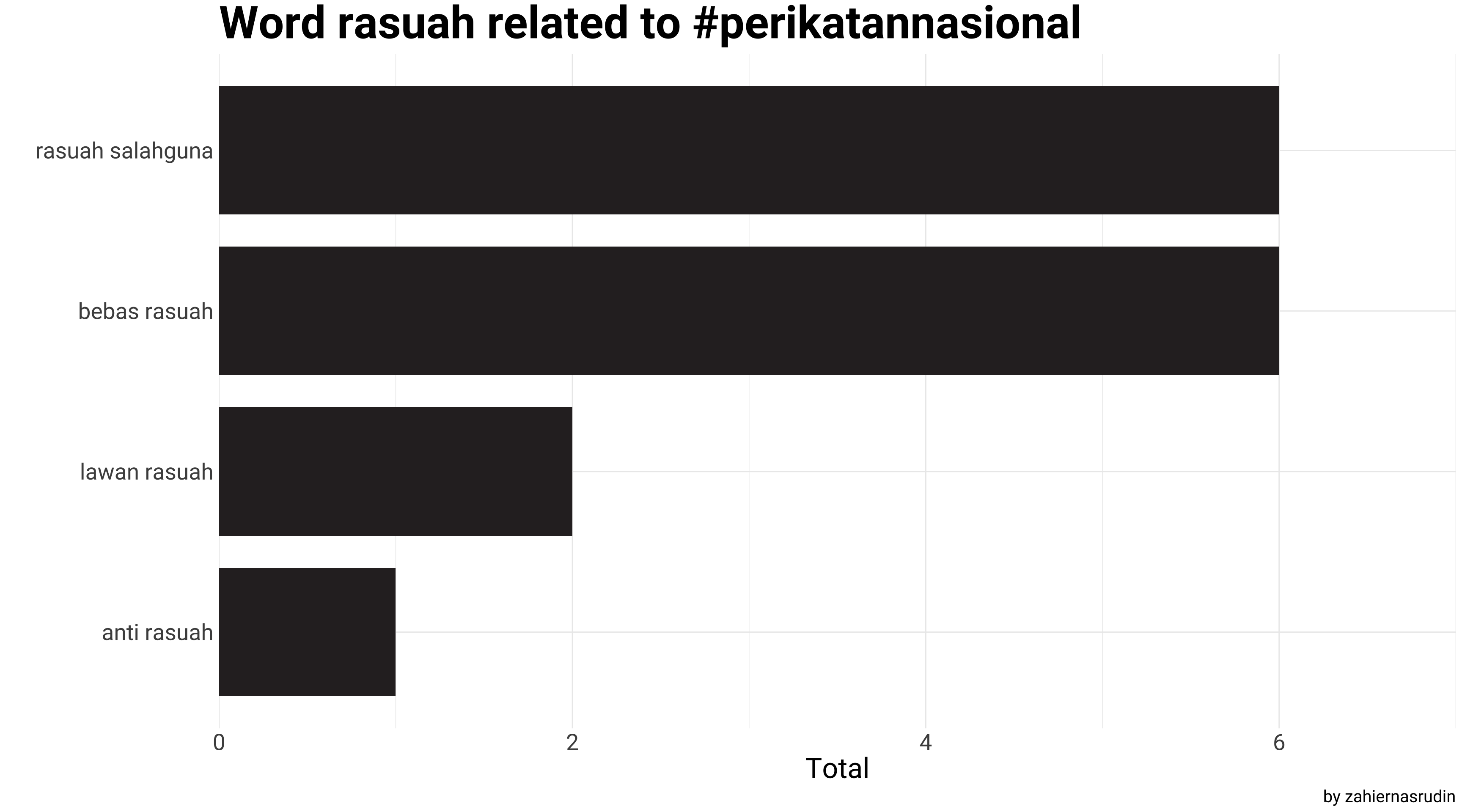
ngram_bn <- bn %>%
mutate(text = remove_url(text),
text = str_remove_all(text, "&|(#[^ ]*)")) %>%
unnest_tokens(word, text, token = "ngrams", n = 2) %>%
count(Party, word, sort = TRUE) %>%
filter(!is.na(word))
ngram_bn_sep <- ngram_bn %>%
separate(word, c("word1", "word2"), sep = " ")
ngram_bn_sep <- ngram_bn_sep %>%
filter(!word1 %in% malaystopwords$stopwords) %>%
filter(!word2 %in% malaystopwords$stopwords)
# new bigram counts:
ngram_bn <- ngram_bn_sep %>%
unite(word, word1, word2, sep = " ")
ngram_bn %>%
filter(str_detect(word, "rasuah")) %>%
group_by(Party) %>%
slice_max(n, n = 4, with_ties = F) %>%
ungroup() %>%
ggplot(aes(x = fct_reorder(word, n), y = n)) +
geom_col(width = 0.8, show.legend = F, fill = "#EDB88B") +
scale_y_continuous(expand = c(0,0), limits=c(0,7)) +
coord_flip() +
labs(x = "",
y = "Total",
title = "Word rasuah related to #barisannasional",
caption = "by zahiernasrudin") 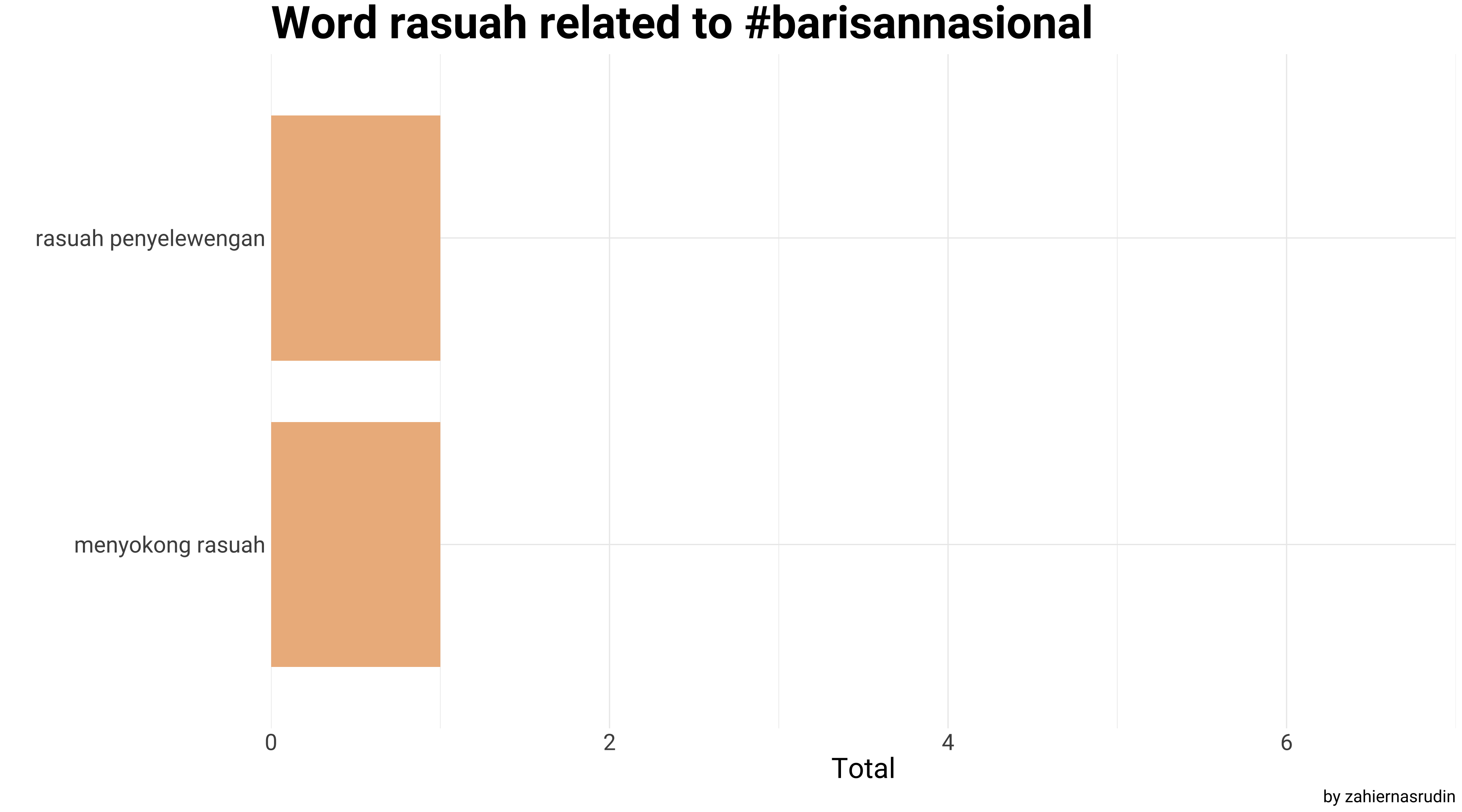
In conclusion, the objective of this project is to evaluate the sentiment of tweets mentioning the hashtags #pakatanharapan, #barisannasional, and #perikatannasional in the lead-up to the 15th General Election of Malaysia. The tweets were first categorized based on these hashtags and the date column was reformatted. We produced a graph displaying the number of tweets; for an overview of the volume of tweets related to these hashtags. Then, a second graph was created to display the number of unique Twitter users mentioning the hashtags, to demonstrate the reach & influence of tweets with these hashtags. The tweets were then split into individual tokens, where we could extract positive and negative words. It was achieved by using malaytextr package, which contains a list of sentiment words. Finally, a graph that displayed the distribution of positive and negative words, giving a clear visual representation of the overall sentiment of tweets. Lastly, we also identified common phrases and expressions that were used in the tweets by using bigrams; and focusing specifically on the word “rasuah” to provide additional insights into the language being used by Twitter users mentioning these hashtags in the lead up to Malaysia’s 15th General Election