ZAHIER NASRUDIN - APS Failure at Scania Trucks

Load library

Code

library(tidyverse)
library(tidymodels)
library(scales)
library(themis)

Load dataset

To begin the analysis, we will be accessing the training and testing datasets for the APS Failure at Scania Trucks project. These datasets are available on the UCI Machine Learning Repository at the following link: https://archive.ics.uci.edu/ml/datasets/APS+Failure+at+Scania+Trucks.

Code

training_set <- read_csv("input/aps_failure_training_set.csv", 
    skip = 20)

test_set <- read_csv("input/aps_failure_test_set.csv", skip = 20)


## Set theme

theme_set(theme_minimal())

Description

Based on the website:

The dataset consists of data collected from heavy Scania
trucks in everyday usage. The system in focus is the
Air Pressure system (APS) which generates pressurised
air that are utilized in various functions in a truck,
such as braking and gear changes. The datasets’
positive class consists of component failures
for a specific component of the APS system.
The negative class consists of trucks with failures
for components not related to the APS. The data consists
of a subset of all available data, selected by experts.

Data exploration

Target distribution

The plot shows the frequency of APS failures, separated by positive and negative class.

Code

training_set %>%
  count(class) %>%
  ggplot(aes(x = fct_reorder(class, n), y = n)) +
  geom_col(width = 0.5) +
  coord_flip() +
  scale_y_continuous(labels = comma, expand = c(0,0), limits=c(0,70000)) +
  geom_text(mapping=aes(label= comma(n), x = class),
            size= 3, hjust = -0.5) +
  labs(x = "Class",
       y = "Total",
       title = "Distribution of APS Failure in Scania Trucks")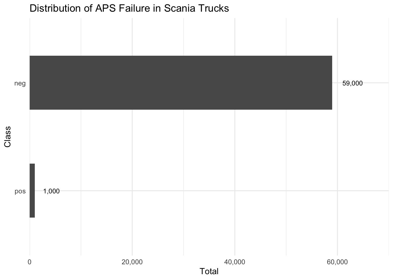

This dataset is heavily imbalanced, with a large majority of negative class points and a small minority of positive class points. To address this issue for this project, we could downsample the negative class points.

Downsampling is a technique, to be used to handle class imbalance in a dataset. In the context of “APS Failure at Scania Trucks” training dataset, downsampling could be applied to reduce the number of negative cases to a level that is more balanced with the number of positive cases. This approach can help to improve the performance of our model on this data, especially if the model is prone to bias towards the majority class (negative)

Missing values

As part of the data exploration process, we would like to get a better understanding of the missing values in our training set. Graph below shows the percentage of missing values in each column. The graph is sorted by the percentage of missing data, with the top 15 columns: with the highest percentage of missing values highlighted. This allows us to quickly discover any columns that may be problematic and plan for strategies to handle missing data.

Code

# Calculate percentage of missing values in each column
missing <- training_set %>% 
  mutate(across(-class, as.numeric)) %>%
  summarise(across(everything(), ~sum(is.na(.))/n())) %>%
  gather(key = "variable", value = "pct_missing")



# Plot the percentage of missing values
missing %>%
  arrange(desc(pct_missing)) %>%
  head(15) %>%
  ggplot(aes(x = fct_reorder(variable, pct_missing), y = pct_missing)) +
  geom_col() +
  coord_flip() +
  geom_text(mapping=aes(label= percent(pct_missing, accuracy = 0.01), x = variable),
            size= 3, hjust = -0.5) +
  labs(x = "Variable", y = "Percentage of Missing Values", 
       title = "Percentage of Missing Values by Column") +
  scale_y_continuous(labels = percent, expand = c(0,0), limits=c(0,1))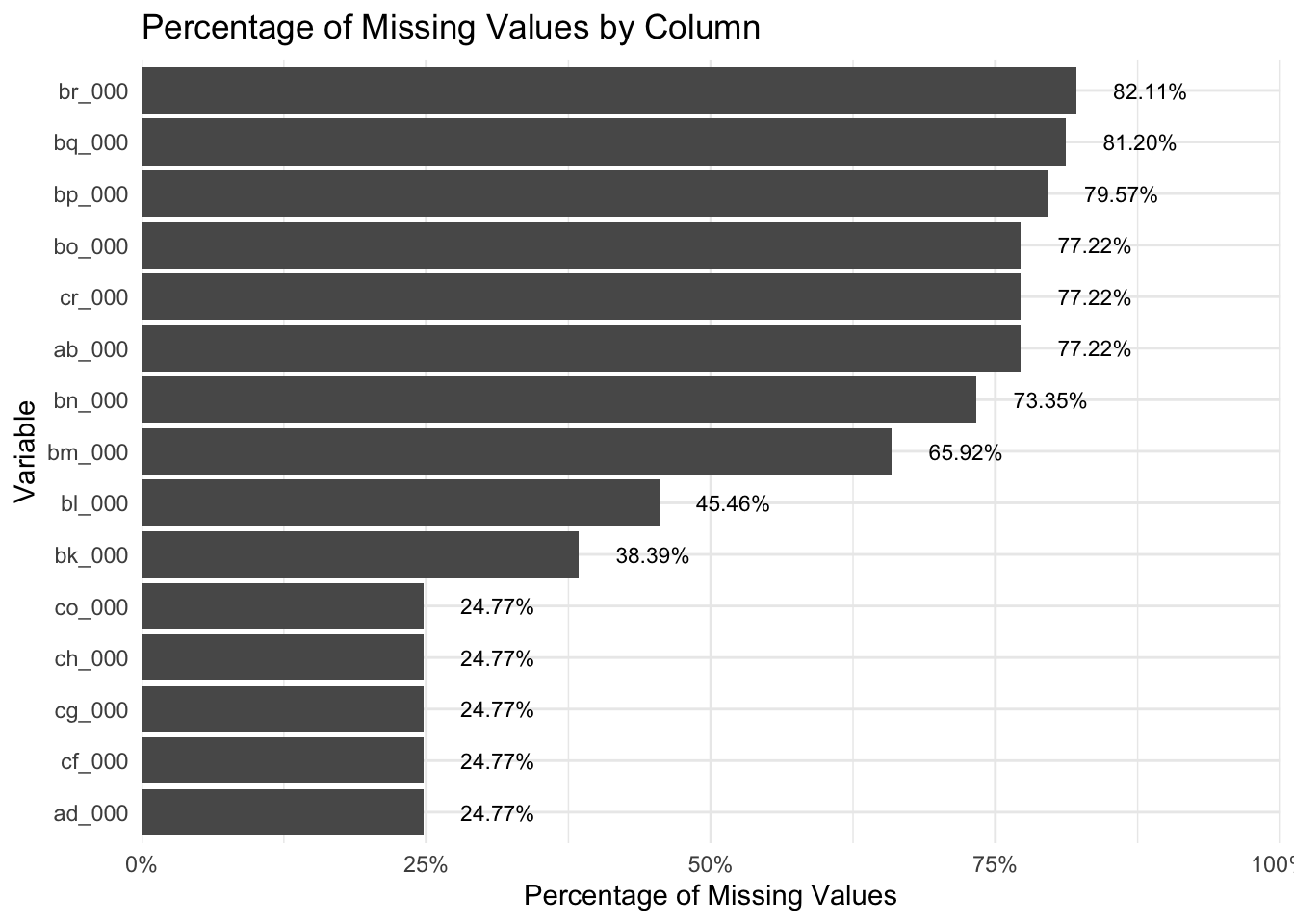

Modelling

Defining recipe

A recipe in tidymodels is a set of instructions for preprocessing and preparing data for modeling. It is a key component of the tidymodels workflow system, which is a package in R that provides a set of tools and interfaces for performing machine learning tasks in a tidy, consistent, and modular way. In this analysis, we are using tidymodels to define a recipe, which is a sequence of steps for cleaning, transforming, and manipulating data in a consistent and repeatable way. To define a recipe, you will need to specify the input data and the specific preprocessing steps that you want to apply to it. This can include tasks such as missing value imputation, feature selection, scaling, encoding, and others.

Our recipe for this analysis:

Removing columns with missing values > 20%
Removing columns with zero variance. Columns with zero variance have the same value for every row in the data, and therefore do not provide any useful information for the model
Transforming categorical variables into a numerical format to be used in our model
Imputing missing values (Using median)
Normalizing columns: Can be useful in a number of situations, such as when the features of the training dataset have different scales or units
Using Principal Component Analysis (PCA). A technique to reduce the dimensionality of the dataset. PCA will help to identify the most important features in the dataset and will be eliminating less important or redundant features, which can make the data easier to understand and analyze.
Downsample negative cases: Can help to reduce the size of a dataset and making it more manageable.

Code

training_set <- training_set %>%
  mutate(across(-class, as.numeric)) 
  


aps_rec <- training_set %>%
  recipe(class ~ .) %>%
  step_filter_missing(all_predictors(), threshold = 0.2) %>%
  step_zv(all_numeric_predictors()) %>%
  step_dummy(all_nominal(), -all_outcomes()) %>%
  step_impute_median(all_predictors()) %>%
  step_normalize(all_numeric_predictors()) %>%
  step_pca(all_predictors()) %>%
  step_downsample(class) 

aps_rec

Model selection

For this project, we will be using Logistic Regression and Support Vector Machines (SVM) as our predictive models to solve classification problem, in this case (negative and positive)

Logistic regression

Code

## Logistic
glm_set <- logistic_reg() %>%
  set_engine("glm")

glm_set

Logistic Regression Model Specification (classification)

Computational engine: glm

SVM

Code

svm_set <-
  svm_linear() %>%
  set_mode("classification") %>%
  set_engine("LiblineaR")

svm_set

Linear Support Vector Machine Model Specification (classification)

Computational engine: LiblineaR

Cross-validation

Cross validation: A technique often used to estimate the generalization error of the models, which would be the error that the models make on new, unseen data.

In our project, we will be applying k-fold cross validation; where the data will be split into k folds, and the model is trained and tested k times. To save time and resources, we are using a 2-fold cross-validation.

Code

aps_fold <- vfold_cv(training_set, v = 2, strata = class)

Define models in a workflow

We will now be using a “tidymodels” workflow to fit logistic regression & SVM models, which allows to easily compare between the two models and also preprocess the data using a downsampling recipe (that we have defined earlier).

Code

aps_models <-
  workflow_set(
    preproc = list(
      all_downsample = aps_rec
    ),
    models = list(glm = glm_set, svm = svm_set),
    cross = TRUE
  )

Fit models

We obtained a sensitivity and an accuracy of more than 95% and a specificity of more than 85% for our models (Logistic regression and SVM); by applying downsampling technique and a 2-fold cross-validation method. These results demonstrate the models are able to identify most of the positive and negative cases; despite the reduced size of the training dataset and a limited number of folds.

Code

set.seed(123)
doParallel::registerDoParallel()

aps_rs <-
  aps_models %>%
  workflow_map(
    resamples = aps_fold,
    metrics = metric_set(accuracy, sensitivity, specificity)
  )


autoplot(aps_rs)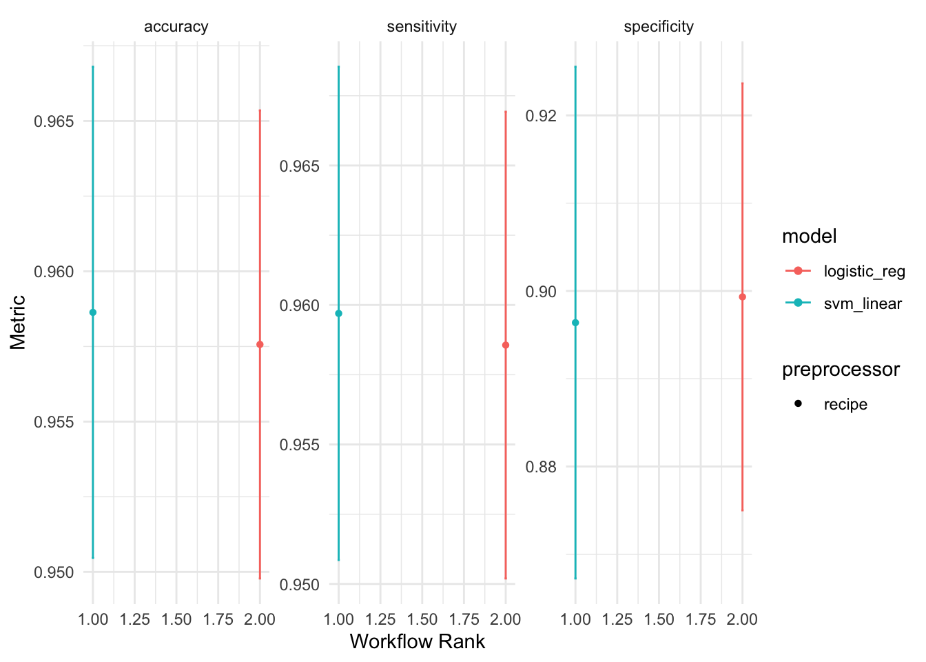

Results by table

We have previously shown comparisons between two models and techniques using chart. We will now be showing the comparisons in a tabular format to make it easier to compare the results.

Code

rank_results(aps_rs) %>%
  filter(.metric %in% c("accuracy","sensitivity", "specificity")) %>%
  mutate(mean = round(mean, 3),
         std_err = round(std_err, 4))%>%
  reactable::reactable(filterable = T, 
                       width = 800)

Train & evaluate final model

After reviewing the performance of our models, we have decided to choose the SVM model over the logistic regression model, as it achieved a slightly higher accuracy, sensitivity scores and very similar specificity score. Although the differences were not very significant, we believe that the SVM model has the potential to provide more accurate and reliable predictions for our data (especially positive cases)

Code

aps_wf <- workflow(aps_rec, svm_set)

aps_fit <-
  aps_wf %>%
  fit(training_set)

Check results on the training set

Code

train_predict <- predict(aps_fit, new_data=training_set) %>%
  bind_cols(training_set)

Confusion matrix

Below is the confusion matrix of the SVM model on the training set. It provides the number of true positive, true negative, false positive and false negative predictions made by the SVM, which could be used to evaluate the model’s performance

Code

train_predict %>%
  mutate(class = as_factor(class)) %>%
  conf_mat(class, .pred_class) %>%
  autoplot("heatmap")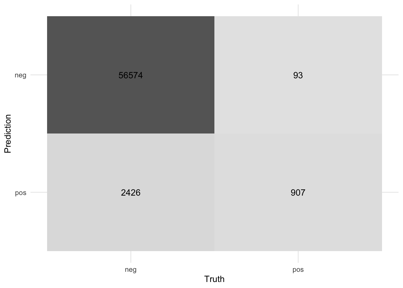

Accuracy, sensitivity, specificity and F-1

The accuracy, sensitivity, specificity, and F1 score of our SVM model can be seen below. The metrics are providing us a summary of the SVM model’s ability to classify negative and positive cases. Based on the metrics, we believe that the SVM model is performing well, considering the simplicity of the model.

Code

train_predict %>%
  mutate(class = as_factor(class)) %>%
  ## Accuracy
  accuracy(class, .pred_class) %>%
  bind_rows(train_predict %>%
  mutate(class = as_factor(class)) %>%
  ## Sensitivity  
  sensitivity(class, .pred_class)) %>%
  bind_rows(train_predict %>%
  mutate(class = as_factor(class)) %>%
  ## Specificity  
  specificity(class, .pred_class)) %>%
  bind_rows(train_predict %>%
  mutate(class = as_factor(class)) %>%
  #F1  
  f_meas(class, .pred_class)) %>%
  mutate(.estimate = round(.estimate, 3)) %>%
  reactable::reactable()

On test data

Having obtained satisfying performance on the training set, we would then apply the SVM model to the test data.

Code

test_predict <- predict(aps_fit, new_data = test_set %>% 
                          mutate(across(-class, as.numeric))) %>%
  bind_cols(test_set)

Confusion matrix

We previously documented the confusion matrix of the SVM model on the training dataset. Below, we are displaying the model’s confusion matrix on the test dataset. These matrices can be utilized to assess the model’s ability to classify unseen cases

Code

test_predict %>%
  mutate(class = as_factor(class)) %>%
  conf_mat(class, .pred_class) %>%
  autoplot("heatmap")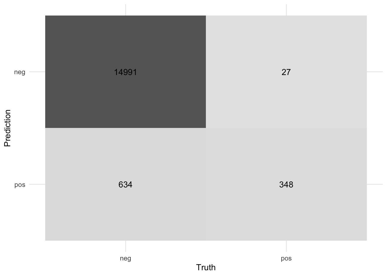

Accuracy, sensitivity, specificity and F-1

Based on the test data,the SVM model performed extremely well, with accuracy, sensitivity, specificity, and F1 score all exceeding 90%. These results demonstrate that the model’s ability to classify a high percentage of both positive and negative cases on the test data, making it a reliable and accurate choice for our application.

Code

test_predict %>%
  mutate(class = as_factor(class)) %>%
  ## Accuracy
  accuracy(class, .pred_class) %>%
  bind_rows(test_predict %>%
  mutate(class = as_factor(class)) %>%
  ## Sensitivity  
  sensitivity(class, .pred_class)) %>%
  bind_rows(test_predict %>%
  mutate(class = as_factor(class)) %>%
  ## Specificity  
  specificity(class, .pred_class)) %>%
  bind_rows(test_predict %>%
  mutate(class = as_factor(class)) %>%
  #F1  
  f_meas(class, .pred_class)) %>%
  mutate(.estimate = round(.estimate, 3)) %>%
  reactable::reactable()

Summary

In this simple project, we used machine learning techniques to tackle the problem of predicting APS failure at Scania Trucks. One noteworthy issue we discovered was that the data was highly imbalanced, with far more negative than positive cases. We chose to downsample the positive cases to address this imbalance.Furthermore, we also used principal component analysis (PCA) to reduce data dimensionality. For the prediction, we used logistic regression and support vector machine (SVM) techniques, and trained and evaluated the models using cross validation with two folds. On the training dataset, both models performed well, with high accuracy, sensitivity, specificity, and F1 scores. Based on the findings, we have chosen the SVM models for our final predictions and presented the model’s confusion matrix on the test data. As a whole, our simple SVM model shows the potential to accurately predict APS failuar at Scania Trucks. In the future, we could compare the results of these models to those of other machine learning techniques, such as Naive Bayes, and also to consider upsampling technique too.